Counterfactual Explanations

Counterfactual Explanations

“You were denied a loan because your annual income was £30,000. If your income had been £45,000, you would have been offered a loan.”

They define Counterfactual Explanations as statements taking the form:

“Score p was returned because variables V had values (v1,v2,…) associated with them. If V instead had values (v1’,v2’,…), and all other variables had remained constant, score p’ would have been returned.”

Adversarial Examples versus Counterfactual Examples

Adversarial Example

• \[x_{adv}=x+\epsilon \times\text{sign(} \nabla f_{x}(x,y)\text{ )}\]
• Invisible to human eyes (see the Figure below.).

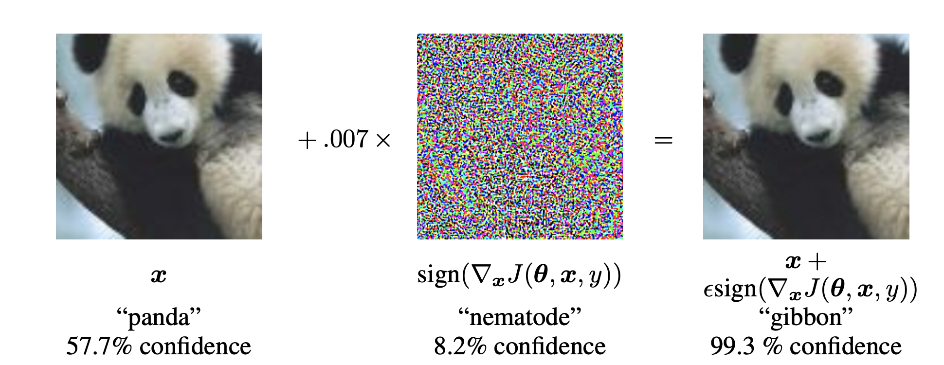(Adversarial Example generated using FGSM method. Img Src. )

Counterfactual Example

• \(x_{c}=x+v\), where \(v\) only modifies few variables to \(x\).

Problem Formulation

Given function \(f: X \mapsto Y\) and \(n\) number of sample points, \((x_1,y_1),\dots,(x_n,y_n)\) sampled i.i.d. from distribution \(P(X,Y)\), for each \((x_i,y_i)\), we want to find the counterfactual example \((x^c_i,y^c_i)\) such that,

1. \(d(x^c_i,x_i) \leq \epsilon\), for some \(d(\cdot,\cdot)\)
2. \(f(x^c_i)=y^c_i\), where \(y_i \neq y^c_i\).

This can be done by solving the following optimization probblem:

Choice of Distance Measure

• Squared Euclidean Distance :

\begin{align} d(x_i,x^c_i) = \sum^d_{k=1} (x_{i,k} - x^c_{i,k})^2 \end{align}

• Scaled Squared Euclidean Distance :

\begin{align} d(x_i,x^c_i) = \sum^d_{k=1} \frac{(x_{i,k} - x^c_{i,k})^2}{std_k(x)} \end{align}

• Scaled L1 Norm :

\begin{align} d(x_i,x^c_i) = \sum^d_{k=1} \frac{|x_{i,k} - x^c_{i,k}|}{MAP_k} \quad \text{where,} \end{align} \begin{align} {MAP_k} = median_j (|x_{j,k} -median_l(x_{l,k})|) \end{align}

Empirical Results

LSAT Dataset

• prediction output : student’s first-year average grade.
• features : race, grade-point average (GPA) prior to law school, and law school entrance exam scores (LSAT).

Counterfactual Question

“What would have to be changed to give a predicted score of 0?”

Squared Euclidean Distance Results

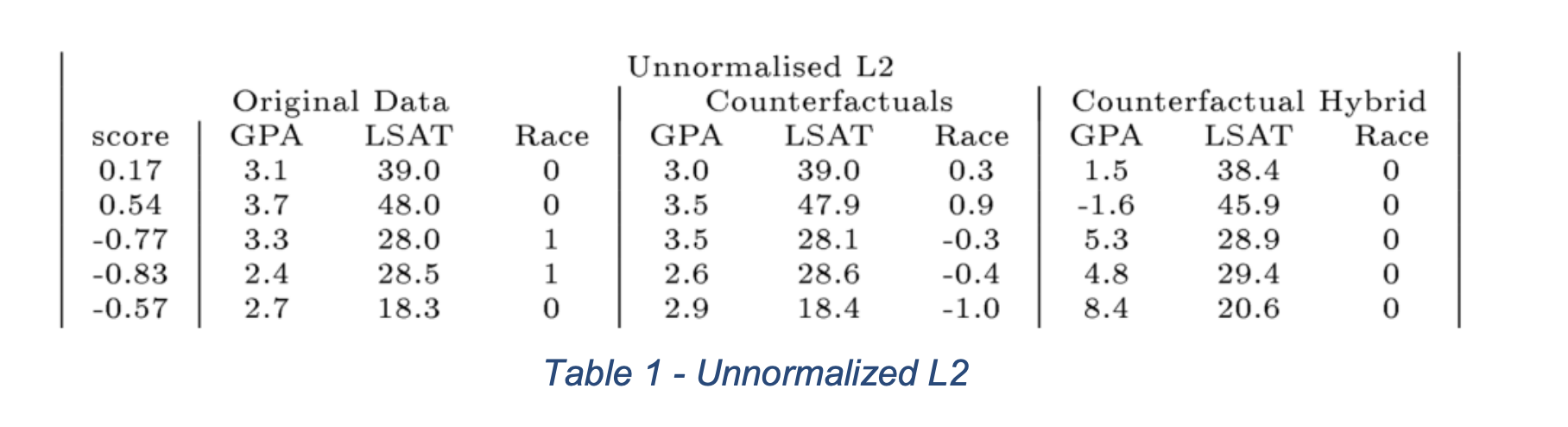(Counterfactual Examples generated using Squared Euclidean Distance. Img Src. )

Scaled Squared Euclidean Distance Results

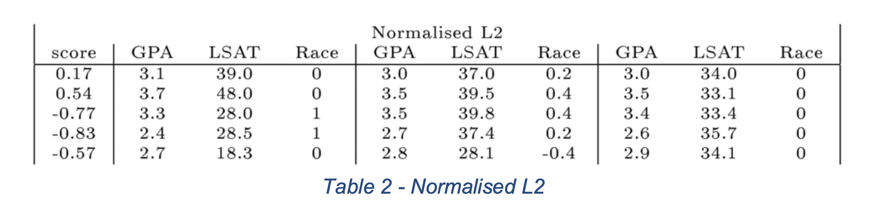(Counterfactual Examples generated using Scaled Squared Euclidean Distance. Img Src. )

Scaled L1 Norm Results

(Counterfactual Examples generated using Squared L1 Norm. Img Src. )

• Person 1: If your LSAT was 34.0, you would have an average predicted score (0).
• Person 2: If your LSAT was 32.4, you would have an average predicted score (0).
• Person 3: If your LSAT was 33.5, and you were ‘white’, you would have an average predicted score (0).
• Person 4: If your LSAT was 35.8, and you were ‘white’, you would have an average predicted score (0).
• Person 5: If your LSAT was 34.9, you would have an average predicted score (0).

Feasibility of Counterfactual Examples (Src.)

Structural Causal Model (Pearl)

A causal model is a triple \(M= <U,V,F>\) such that \(U\) is a set of exogenous variables, \(V\) is a set of endogenous variables that are determined by variables inside the model, and \(F\) is a set of functions that determine the value of each \(v_i \in V\) (up to some independent noise) based on values of \(U_i \in U\) and \(Pa_i \in V\) \ \(v_i\).

Global Feasibility

Let \(<x_i,y_i>\) be the input features and the predicted outcome from \(h\), and let \(y'\) be the desired output class. Let \(M=<U,V,F>\) be a causal model over \(\mathcal{X}\) such that each feature is in \(U \cup V\). Then, a counterfactual \(<x^{cf},y^{cf}>\) is global feasible if i) it is valid \((y^{cf}=y')\), ii) the change from \(x_i\) to \(x^{cf}\) satisfies all constraints entailed by the causal model, iii) and all exogenous variabbles \(x^{exog}=U\) lie within the input domain.

Generative Model

\begin{align} \bullet \Pr(x^{cf}|y’,x) \quad \text{such that } x^{cf} \text{ belings to class } y’ \end{align}

\begin{align} \bullet \text{ encoder} \quad q(z|x,y’) \end{align}

\begin{align} \bullet \text{ decoder} \quad p(x^{cf}|z,y’,x) \end{align}

Evidence lower bound (ELBO)

\begin{align} \ln{\Pr(x^{cf}|y’,x)} \geq \mathbb{E}_{Q(z|x,y’)} \ln{\Pr(x^{cf}|z,y’,x)} - \mathbb{KL}(Q(z|x,y’||\Pr(z|y’,x))) \end{align}

Approximation

Causal Distance

Given causal graph \(G\) over \(U\cup V\) and mechanisms \(F\), for each \(v \in V\), we have \(v=f(v_{p1},\dots,v_{pk}) + \epsilon\), where \(\{v_{p1},\dots,v_{p_k}\}\) are the parents of \(v\). We can define the \(Distance\) for the nodes \(v \in V\) as follows:

For the nodes \(u \in U\), we can use L1 or L2 distance measure. We can now define the distance measure as follows:

References

• Counterfactual Explanations without Opening the Black Box: Automated Decisions and the GDPR
• Explaining and Harnessing Adversarial Examples